|
PIAS Manual
2026
Program for the Integral Approach of Shipdesign
|
|
PIAS Manual
2026
Program for the Integral Approach of Shipdesign
|
If a compartment is damaged in such a way that it is open to sea water then it will obviously be flooded, which can also extend further into the vessel through all kinds of connections between compartments. In stability regulations, the word progressive flooding is sometimes used for this, but we rather avoid this word because it suggests that the flooding continues until it is fatal, which of course is not necessarily the case. Obviously, this process can be modelled in PIAS and computed. There are two facilities for this purpose:
The choice between these two systems can be made in Config (or through Project Setup in the upper bar of the PIAS window), Please also refer for this setting to Calculation damage stability according to the method of, which also contains a list of PIAS features and functions which are disabled in combination with Consecutive Flooding.
This chapter discusses the following:
This system is discussed in the four sections below, viz.:
This order may appear to be a bit unnatural — because we should first define, before being able to use — but is nevertheless deliberately chosen this way. By the way, before doing any calculations, one will of course have to define the ducts and pipes. This is done integrated with bulkheads, decks and compartments, in Layout, as described in Pipe lines and piping systems.
This method was conceptualized given two facts:
In the elder “compartment connection” method of PIAS the latter was facilitated by so-called “complex stages of flooding”, which support individual percentages of flooding for different compartments. This offered full freedom, however at the cost of significant manual input labour. For the numerous damage cases of probabilistic damage stability this is not practical, so module Probdam offered a specific feature to generate these complex stages, where the binary concepts of “open” and “pipe” (as discussed in Damage cases generation including "progressive flooding") offered a flexibility sufficient for the majority of cases, but not for all cases. So, in the consecutive flooding system a novel subsystem for unequal intermediate stages of flooding has been created which is a) flexible, b) based on generation so does not require much user input, and c) works for all PIAS damage stability calculation modules.
This subsystem maintains the notion of “percentual stage of flooding”, because a) this is a fundamental concept in present damage stability regulations, b) therefore this concept is familiar to authorities and classification societies and c) the concept is easy to understand. In order to have a shorthand word for this concept it was labelled “fractional”, because essentially it fills compartments by ‘fractions’ of the final volume. So that fraction is the unit, which enables us to introduce an integer “delay” in the flooding of connected compartments. Assume, for the time being, that the percentages of flooding are 0, 25, 50, 75 and 100%, so one fraction corresponds with 25%. If we use a delay of zero (so, no delay), then the flooding of a connected compartment will obviously be the same as for the ruptured compartment:
| Fraction ruptured compartment | Fraction connected compartment |
| 1 (=25%) | 1 (=25%) |
| 2 (=50%) | 2 (=50%) |
| 3 (=75%) | 3 (=75%) |
| 4 (=100%) | 4 (=100%) |
With a delay of 1, there will be a single fraction delay:
| Fraction ruptured compartment | Fraction connected compartment |
| 1 (=25%) | 0 (=0%) |
| 2 (=50%) | 1 (=25%) |
| 3 (=75%) | 2 (=50%) |
| 4 (=100%) | 3 (=75%) |
| 4 (=100%) | 4 (=100%) |
The last row is added because the filling should always end up with all flooded compartments filled to their final levels.
And with a delay≥4:
| Fraction ruptured compartment | Fraction connected compartment |
| 1 (=25%) | 0 (=0%) |
| 2 (=50%) | 0 (=0%) |
| 3 (=75%) | 0 (=0%) |
| 4 (=100%) | 0 (=0%) |
| 4 (=100%) | 1 (=25%) |
| 4 (=100%) | 2 (=50%) |
| 4 (=100%) | 3 (=75%) |
| 4 (=100%) | 4 (=100%) |
This was an example of a single connection between two compartments. But also cascaded connections are supported by nature, take for instance this configuration of three compartments and two connections (with each a delay of 1):
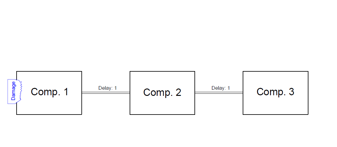
| Fraction comp1 | Fraction comp2 | Fraction comp3 |
| 1 | 0 | 0 |
| 2 | 1 | 0 |
| 3 | 2 | 1 |
| 4 | 3 | 2 |
| 4 | 4 | 3 |
| 4 | 4 | 4 |
Also more complicated topologies are allowed. The delay factors for the different paths might contradict, but that poses not a real dilemma, because the smallest fraction determines the actual flooding, which is a sound logical consequence of the underlying assumptions. For example this case:
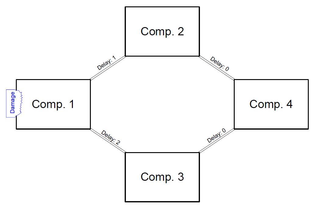
| Fraction comp1 | Fraction comp2 | Fraction comp3 | Fraction comp4 |
| 1 | 0 | 0 | 0 |
| 2 | 1 | 1 | 1 |
| 3 | 2 | 2 | 2 |
| 4 | 3 | 3 | 3 |
| 4 | 4 | 4 | 4 |
Initially the fraction sequence for Comp3 appeared us to be 0,0,1,2,3,4 but through Comp2 and Comp4 the compartment fills up faster.
Delay factors are given for each pipe segment (which is a connection between two joints or compartments, without any branch inbetween, see Segment list)). That enables a pipe topology and delay factors such as:
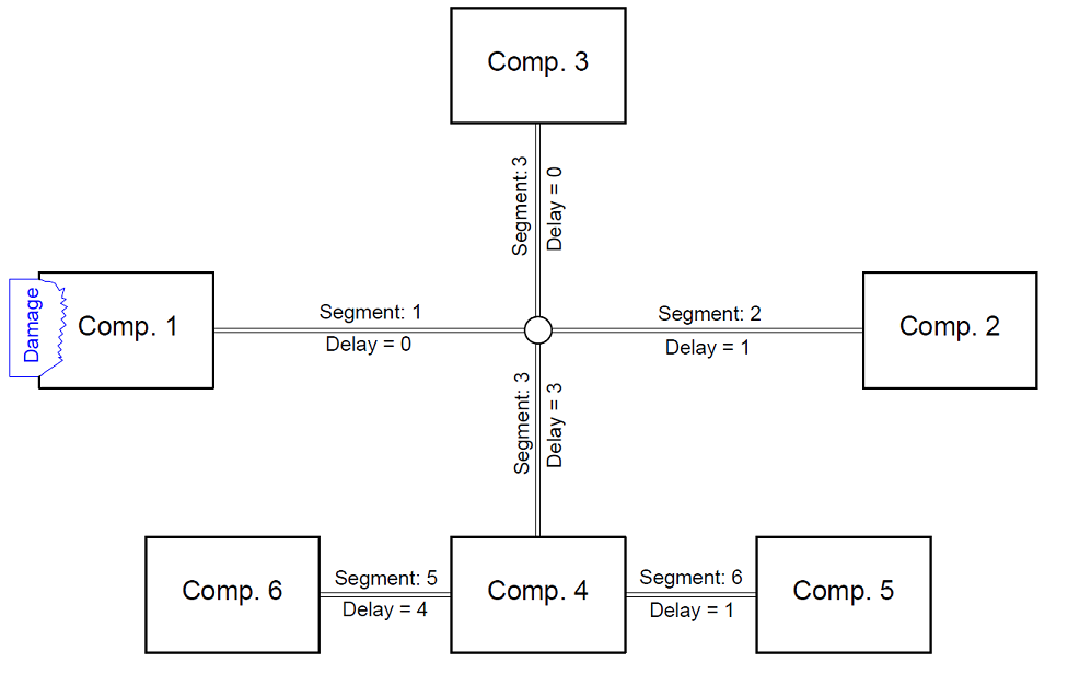
Which will lead to eleven different stages of flooding (including the final stage).
That's the basic idea. And how realistic will modelling method be? Just as realistic as the whole presumption of fixed percentages of flooding, as imposed by all major damage stability rules. For added flexibility PIAS goes one step further, by allowing multiple (to a maximum of three) delay factors per pipe segment. In most cases a single delay factor will suffice, but even more complex scenarios than presented in this section can be modelled with combinations of factors.
Finally, a remark on the percentages of flooding as used in the examples of this section. As demontration, multiples of 25% have been used, but you will certainly be aware that in PIAS the number of intermediate stages of flooding is user-defined, as well as the percentage of each stage. So, where we have used multiples of 25% here, in reality for this percentage the user-defined flooding percentages will be applied.
A calculation in the time domain involves analysing, for a whole series of small time steps, how fluids flow through pipes and openings and how that effects ship's position and stability. That is essentially a model which is based on physics, and therefore needs much less explanation than the fractional method, which is a bit artificial. Nevertheless, some choices and assumptions have been applied here and there, which are discussed in Basis of damage stability in time domain.
The piping geometry and connectivity can be defined in combination with the internal (i.e. compartment) geometry, with module Layout. This is discussed in Pipe lines and piping systems. In order to keep data of the same categories as much together as possible, the flow-related choices and parameters will be discussed in this section.
Frictional resistance through pipes is in the essence a complex issue. In practice, however, there are a number of practical methods and parameters in use, and in PIAS we have chosen to implement a selection:
The resistance of fluid flowing through a pipe consists of two components. One is the frictional or possibly pressure resistance in the pipe, and the other one is due to the energy loss of the fluid outflow at the pipe outlet. The latter one simply follows from the fact that the fluid travels with some velocity through the pipe, and hence carries kinetic energy. After outflow (into a reservoir, or into the open air) that velocity vanishes, so the energy content also has gone. This is inevitable, also in a frictionless world. This phenomenon should be included — once, not twice. Unfortunately the different IMO regulations are not consistent in this respect. There are three IMO regulations involved, res. A266 (1973), MSC. 245(83) (2007) and MSC. 362(92) (2013). In A266 and 362 this outflow loss is included implicitly, while in 245 a energy loss factor should be included explicitly, in combination with frictional resistance coefficients of the piping configuration.
PIAS offers you this choice. It can be given in a user setting, in Layout, labelled ‘Processing of outlet losses’ (please see General piping settings), with binary choice ‘Explicitly user-defined by means of resistance coefficients’ or ‘Implicitly taken into account’. Please ascertain to set this switch in accordance with the resistance coefficients you assign to the pipe line components, and with this background in mind:
When assessing the damage stability with a cross flooding device, the question may arise which stability criteria to apply; those for final stage or those for intermediate stages of flooding? PIAS' consecutive flooding system has two mechanisms for this, one for the fractional intermediate stages and one for the time domain calculation.
In the essence, the application of intermediate or final criteria depends on the time span of the filling process. Some regulations (or accompanying explanatory notes) therefore contain a maximum time period until equalization. This implies that if the ship does not equalize within that time, the cross-flooding arrangement is deemed ineffective, so stability in the non-equalized condition is considerd to be a final stage, which should meet the final stage stability criterla. Well, the whole concept of equalization might apply to two simple interconnected tanks on either side of centerline, but for a slightly more complex tank arrangement, it is an abstraction that is not so easy to relate to reality. Nevertheless, the underlying idea is easy to transform into a universal algorithm:
To this end, that maximum time allowed must be given, which can be done in the general settings for damage stability, see General settings damage stability.
Above, we have seen that with the time domain calculation, the criterion choice can be elegantly linked to an equalisation time, but for a calculation with conventional intermediate stages of flooding the time information is missing. To allow the user to influence this, PIAS has a facility to specify whether a pipe is large or small. These concepts ‘large’ and ‘small’ have no numerical relationship to the pipe size, but only to the choice of stability criteria to be applied, in this fashion:
The size, large or small, of a cross section can be specified as a general piping setting (see General piping settings) with exceptions per network where applicable.
For the purpose of damage stability calculations, many properties of pipe components can be specified, such as dimensions and coefficients. Because many pipes will be similar it can happen in practice that one is typing in the same numbers over and over again, and nobody likes that. In order to increase the ease of use, PIAS is therefore equipped with the feature to specify some of those parameters in ‘layers&rsquo. So, a parameter can explicitly be ‘not specified’, which will make PIAS to look for the corresponding parameter in a higher layer.
Clearly, this system is designed to minimize user input. So, one can specify a default at a higher level (e.g. at the level of a piping system) and leave all the items below it set to ‘not specified’, hence corresponding to the default. Only the exceptions then actually have to be given individually.
As can be read in this chapter, Consecutive Flooding is controlled by quite a few settings and parameters. Because these are given in various places in PIAS, the impression may arise that there was no sharp plan behind this when developing the software, but this is by no means the case. Some parameters simply belong to a physical thing — a pipe or a valve — and hence to its definition in Layout, while others are calculation parameters which belong to the general settings for damage stability calculations, or to a specific piping network. Anyway, to provide the user with an overview, the several settings are summarised in the table below.
TODO make summary in table
Preliminary remark: as mentioned in the introduction to this chapter, PIAS now has two systems that can be used to account internal flooding between compartments. The subject of this section's system, complex intermediate stages, was in development until ±2020, after which development has focused on the more advanced Consecutive flooding system, see Flooding through ducts and pipes: Consecutive Flooding, after 2022.
This section a number of distinct facilities will be discussed:
In each module for damage stability of PIAS, with the exception of the computation of floodable lengths, damage cases are defined at least by defining which compartments will be flooded for that case. This is discussed at Input and edit damage cases, where in the menu bar the [Flooding stages] function is included. When this fuction is used the following option menu appears:
The first option in this menu concerns the calculation type. There are two types of calculation:
After selecting this option the following input screen appears which contains all damaged compartments:
| Damage case ABC | |||||
| Compartment | Connected with | Via critical point | |||
| Length | Breadth | Height | SB&PS | ||
| DEF | - | - | - | - | - |
| PQR | Seawater | 10.123 | 8.123 | 6.123 | Yes |
| STU | PQR | 23.123 | 8.123 | 6.123 | No |
| XYZ | STU | 43.123 | 8.123 | 6.123 | No |
A critical point defines an internal opening between two damaged compartments. The compartment will only then be flooded (with the percentage of flooding in a certain intermediate stage) when the level of liquid of the compartment in ‘Connected with’ is higher than the critical point. When for a critical point the column ‘SB&PS’ is set to ‘Yes’, than that point exists on SB and on PS (with an equal breadth from CL). The same mechanism is applicable to critical points if ‘Connected with’ is set to ‘Seawater’.
The mechanism contains three limitations:
With the text cursor on a specific compartment, and pressing <Enter>, the next input screen appears in which the percentage of filling for a certain intermediate stage of flooding for that compartment can be defined, for example:
| Compartment XYZ | |||
| Stage Number | Percentage of flooding | Water on deck | Stab.crit.final |
| 1 | 25 | No | No |
| 2 | 50 | No | No |
| 3 | 75 | No | No |
| 4 | 100 | No | No |
| 5 | 100 | No | No |
| 6 | 100 | No | Yes |
A calculation with all compartments filled with 100% does not have to be defined, because this is the final stage of flooding which is calculated automatically.
According to the rules of the ‘Agreement concerning specific stability requirements for Ro-Ro passenger ships undertaking regular scheduled international voyages between or to or from designated ports in North West Europe and the Baltic Sea’ (Circular letter 1891), as adopted on 27-28 February 1996. A.k.a. as ‘Stockholm agreement’ and by EU directive 2003/25/EC 2003 also applicable to amongst others the Mediterranean. The core of the regulations is an additional amount of water on deck, dependant on the residual freeboard. To include the effects of water on deck:
This calculation type is aimed at the very simple case of a compartment connected to sea water via a pipe or hole which has fluid flow resistance. Much more complex systems of pipes and connections can be addressed with Consecutive Flooding, see Background from tools for ship-internal connections in PIAS.
After chosing this calculation, a list of compartments is presented, where for each compartment can be specified:
In the output of the deterministic damage stability (with Loading) with complex intermediate stages, the percentage of flooding is not printed in the heading but in the table with weights per compartment. For the intermediate stages of flooding of the computations of maximum allowable VCG' (as discussed in Maximum VCG' damaged tables and diagrams) only the number of the intermediate stage is printed.
The method of damage stability calculations is largely fixed by rules and conventions, and obviously this forms the basis for the implementation in PIAS. However, there are also a number of issues that are less clearly elaborated — such as the question of what exactly is the amount of fluid corresponding to a certain percentage at an intermediate stage of filling, or how to deal with a small internal opening when calculating the stability curve. The choices as made for such issues in PIAS are discussed below, for the two available systems:
The elder method is based on intermediate stages of flooding, and the newer one also includes a sub-method on that basis. However, the two do differ slightly, which is discussed in Difference in principles at intermediate stages.
By the way, while searching through decades-old documentation for the program approval by classification societies, we still came across the phrase that the damage stability calculation of PIAS includes the free-to-trim effect. A bit overdone to repeat that message, but just to be sure: it still does, also with Consecutive Flooding.
Here we discuss the effects that the internal connections and its components have on the calculations of intact and damaged stability, when using the system of Consecutive Flooding.
The whole assumption behind the idea of a fraction (a generalization of an intermediate stage of flooding, see With conventional intermediate stages of flooding ("Fractional")) is that the immediately affected compartments will be flooded through a small damage. After all, if the damage were large, the ingressed water would spread rapidly, and the intermediate stage would be so short that it would have no effect on ship's position and stability. So, then the intermediate stage would actually not exist. Based on this physics-based reasoning, a distinction is made between large and small damages.
To assess stability in damaged condition, the worst-case scenario will have to be considered and since it is not known in advance how large the damage will be, cases with both a large and small damage are calculated.
In the event of large damage, seawater can flow freely in and out of the affected compartments, so that even during roll the water level in those compartments is equal to the sea water level. Because this all happens so quickly, intermediate stages do not actually emerge.
In the case of a small damage, on the other hand, the water flows through the hole so slowly that the intermediate stages can take a long time, and thus should be considered separately. However, if the water flows slowly, then during rolling it does not have time to flow in and out significantly. So, in this case the volume of water in a compartment can be assumed to be constant for all heeling angles.
The percentages of the stages of flooding can be set by the user, this is discussed in Define stages of flooding. Suppose intermediate stages of 25, 50 and 75% are given, then the complete damage stability evaluation will consist of:
| Damage | Stage | Water in compartiment | Verified against stability criteria for |
| Large | Final | Freely flowing in and out | Final stage |
| Small | Final | Constant, as at equilibrium angle (call that W) | Final stage |
| Small | Intermediate | 75% from W | Intermediate stage |
| Small | Intermediate | 50% from W | Intermediate stage |
| Small | Intermediate | 25% from W | Intermediate stage |
So, this intermediate-stage system is governed by the size of the damage. However, one could argue that the size of further internal openings (or pipelines or other connections) will also play a role. Indeed, this effect on the computation of the GZ-curve is discussed in Basis of larger angle stability (GZ-curve). Additionally, the sizes of the internal connections also determine the choice of the damage stability criteria to be applied. Also in this area PIAS gives influence to the user, which is discussed in Choice of stability criteria with the fractional method.
The whole idea behind the time domain method is that the vessel gradually fills up through openings and pipes and so on. With each time step subdivided in these sub-steps:
This is somewhat simplified — e.g. additional analyses take place, such as checking whether the points of a pipe segment are all below the liquid level, if not the segment flow is blocked — the process, which the user can control by e.g.:
In principle, at each of the time steps, the (damage) stability could be calculated, but that would lead to abundant output. Therefore, there are handles that allow the user to limit those time steps, see Time domain calculation time step and Minimum weight difference for a GZ calculation. At the time of such a stability calculation, the fluid content (generally consisting of a mixture of intact content and ingressed sea water) is held constant, and a stability calculation is made according to the same principles as with “fractions” (see Basis of larger angle stability (GZ-curve)). Actually a rather simple mechanism. ALthough there are still a few more details worth mentioning:
In Basis of damage stability with fractions ("intermediate stages of filling"), it has been plausibly shown that a small damage results in the volume of the compartment located behind the damage can be assumed constant during heel, whereas with a large damage the fluid can flow in and out freely during heel. Exactly the same reasoning applies to internal connections, holes and pipes. This treats internal connectionss in the same way as the damage, albeit that with the damage, since only one of these is assumed, a worst case scenario with combinations of small and large damages can be drawn up. Internal connections, on the other hand, can be numerous and it would take large amounts of computing time to start calculating all kinds of combinations of large and small from them. Therefore, for the internal connections, it was chosen to have the demarcation between ‘large’ and ‘small’ set by the user, which was discussed atconfig,config_damage_stability_CFminarea}. In short, if the cross-sectional area of a connection is larger than this value, then the fluid flows freely through that connection during heel, and otherwise not.
By the way, it will be obvious that due to sudden fluid transfer between heeling angles, the GZ curve will not always be nice and smooth. Traditionally, the GZ (plus associated draft and trim) is calculated at a fixed series of angles (of, e.g. 5°, 10°, 20°, 30° etcetera) but this does not model discontinuities in the GZ curve properly. After all, it will make a difference when fluid flows over an internal threshold at 21° or at 29°. Therefore, in Consecutive Flooding the GZ calculations are done at many more angles, in the order of every degree. To limit the output in loading and damage calculations, only the angles set at Angles of inclination for stability calculations are printed from these. Obviously, this larger angle range will increase computation time correspondingly; that is the price to pay for the increased accuracy. A small price, because PIAS has quite a few features (see Speed enhancing mechanisms in PIAS: PIAS/ES) that can speed up series of (damage) stability calculations by several times.
The application of Consecutive Flooding is not limited to damage stability; also in intact conditions a compartment will be flooded through a submerged opening connected by a piping system. While that could be an interesting possibility, the practical importance of this is so small that it will not be included in PIAS for now.
The method of calculation in intermediate stages of flooding is simple in the essence, with the following steps:
This scenario will not always represent reality, but it is the best fit for the dogma of the “fixed percentual intermediate stage of floodingt”. Those who do not agree with this approach will have to choose a more adequate scenario, e.g. a calculation in the time domain.
Two more details are worth knowing about the calculation method:
Both the elder (pre-2023) damage stability calculation system, and the Consecutive Flooding system contain calculations with intermediate stages of flooding. Perhaps one would expect their results to be the same, but that will by not always be the case. This is not so surprising, as both methods have their own calculation bases. The details of these have been discussed in previous sections, but in summary they boil down to this:
One might ask which method is best. In general, that question cannot be answered. After all, the first method has the advantage of elegance, adding that many thousands of such calculations have been approved by classification societies and Shipping Inspectorates over the past decades. While the second method has the advantage that diverse configurations with varying sizes of damages, openings, pipe lines, holes and connections rest on a certain physical foundation. Because Consecutive Flooding supports just such a large variety, it was necessary to switch to the second method for that.
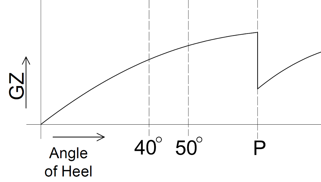
How does PIAS deal with an internal threshold or pipe which is submerged, and hence allows transfer of water, at an angle of heel which is beyond the static equilibrium? Take for example the GZ-curve as sketched below, where at angle P the upper edge of a partial bulkhead overflows, leading to the filling of an adjacent compartment and hence a deteriorated stability. It will be undebatable that the GZ will initially follow curve A, until angle P is reached, where a greater amount of ingressed water will lead to reduced curve B. However, the question is what happens on the “way back”, i.e. with decreasing angle of heel? The water will not fully flow back over the bulkhead, so a curve more or less as indicated by C can be expected. And the subsequent question is which curve to use for the verification of GZ against stability criteria, A+B or C+B?
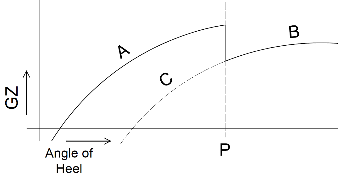
In PIAS the past decades A+B has always been used — numerous calculations have been issued at classification societies and shipping inspections, and approved — based on the reasoning that the notion “way back” is never properly addressed, neither in literature nor in regulations. A few more arguments can be made in favour of this choice:
Supported by these arguments, it was — in 2022, during the re-evaluation at the introduction of consecutive flooding — chosen to keep the computation method for this subject in PIAS as it always has been. Please understand that this is an implementation choice, not the irrevocable result of the modelling method in PIAS. So alternative choices could be made, if there would be a reason for that, such as a generally accepted convention. Other reasons could be clear and unambiguous guidance by rules or regulations or unified interpretations from institutions, such as IMO, IACS or national authorities.