|
PIAS Manual
2026
Program for the Integral Approach of Shipdesign
|
|
PIAS Manual
2026
Program for the Integral Approach of Shipdesign
|
At start up a progress bar in the status bar indicates how solids are read into the GUI. This process is completed when it reads “Ready” in the status bar, and the GUI is responsive to the mouse and keyboard. Curves are represented by a course polyline initially in order to get ready for user interaction quickly, and the system continues preparing for final display accuracy and the curvature information while the user is working with the model. Care is taken that curves that are under the mouse pointer are prioritised, so that these are always displayed at high accuracy. Because of this task, CPU load can be high for the first moments after loading a large model, but it will normalize eventually. For configuration of the display accuracy see Configuration GUI.
The GUI consists of a central modelling area, around which various control- and information panels can be positioned, according to the preferences of the user. The menu bar along the top and the status bar along the bottom are the only static elements in the main window, everything else can be repositioned, detached and embedded by means of drag-and-drop. To show or hide a particular window, click on the corresponding item in the [Window] menu.
The modelling area can be filled with one or more modelling views in various layouts. A new modelling view can be opened with [Window]→[new]. When there are several views open in the modelling area, the one under the mouse pointer is automatically activated and raised to the front in case of overlapping views. A view can be prevented from being occluded by the active view by selecting “Stay on Top” from the drop-down menu under the top left icon of the view window. View windows may be layed out automatically filling the modelling area by selecting [Window]→[Tile].
As Fairway has excellent controls for changing the view angle and zoom level in a view window (see Navigation: Pan, Zoom and Rotate) many people prefer working in a single maximized window, which you get by clicking on the corresponding button in the top right corner of the view window frame. Alternatively, several large views may be stacked on top of each other by selecting [Window]→[Stack]; which gives each window a tab pane along the top for switching between views.
The projection of the view can be toggled between parallel projection and perspective projection from the context menu, by clicking the right mouse button over the view window in question. Since manipulation of curves in various planes is very well handled in Fairway and independent from the view angle or projection, you may even prefer to model and manipulate in perspective, as it helps with spatial orientation and to differentiate curves in the foreground from the rest of the model; it is a depth cue.
When the GUI is closed, the view window layout and view angles are stored and restored when the GUI is reopened at a later time.
The tree view contains a hierarchical list of the elements of a model. It can be shown and hidden from the menu [Objects]→[Tree View], and be repositioned to another location — even another screen if you have one — by dragging its title bar. A double-click on the title bar toggles between floating above the main window and embedded within.
The tree can be expanded and collapsed by clicking the small triangles to the left of the items, or by double clicking the item itself. To expand an item and all its sub-items, select the item and press <*>. Every solid has a sub-item for visualisation of its shell surface, followed by sub-items for every kind of polycurve.
Solids appear as the top-level elements in the tree view. A solid can be hidden or shown by toggling the check box in the Visibility column, or changed between active and inactive by toggling the check box in the Access column. An inactive solid cannot be manipulated, which is indicated graphically with a uniform colour. When a solid is hidden it is automatically made inactive, and when a solid is activated it is automatically made visible. These changes are recorded in the action history and can be undone, see Undo and redo.
The order of solids in the tree view kan be changed by bringing up the context menu with a click on the right mouse button and the option [Relocate in tree]. This change is saved with the model, but since it has no implication on the action history it cannot be undone.
Whether or not the solid is buoyant can also be changed using the context menu. This change can be undone.
The visualisation of the shell can be toggled for each solid individually with the check box behind the [Shell] item. To reveal or hide the shells of all solids at once, the [Show All Shells] and [Hide All Shells] buttons in the [Display]→[Rendering...] window can be used. That window also contains the options with which the visualisation of the shell can be adjusted.
The [Shell] item can be expanded to reveal the [Material] properties. Both the color and transparency of the surface can be changed here with a double-click on the corresponding value. However, the shell of inactive solids is rendered uniformly as set in [File,Preferences...,Curves,Solids,Inactive color].
Changes to the shell visualisation settings in the tree view are saved with the model, but they are not recorded in the action history as they do not affect modeling actions. The settings in the [Display]→[Rendering...] window are user preferences and are thus shared across projects.
When a polycurve is selected graphically, the tree is automatically expanded and scrolled to bring the selection into view. Selections can also be made in the tree view with the left mouse button <LMB>. A composed selection is made with <Ctrl+LMB> and a range is selected with <Shift+LMB> or holding <LMB> while dragging over the list. It is also possible to select all expanded items with <Ctrl+A>. A click with the right mouse button on a polycurve in the tree view brings up the context menu from which the polycurve can be renamed, and actions on that particular polycurve can be started.
There are two additional columns in the tree view containing check boxes for visibility (see Polycurve visibility) and access (see Polycurve locked). If a particular polycurve is hidden, the visibility check box of its parent item as well as of its parent solid is filled to indicate that not all polycurves are visible. Clicking this box in the parent solid will unhide all polycurves in the solid. Clicking this box in the parent item unhides all child polycurves if there are hidden polycurves, otherwise it hides all of them. The menu option [Display]→[Unhide All] will unhide all hidden items in the entire model at once.
The Access column controls the active/inactive state of solids, and the lock status of polycurves. Inactive solids change to a uniform colour and cannot be modified. Polycurves can be in one of three lock states:
An irremovable polycurve can still be modified, but not be deleted. The polycurve lock state is cycled with a click on its check box.
State changes are recorded in the action history and can be undone and redone, see Undo and redo.
Polycurves always have at least one child curve. Its name indicates the type of the curve and a running number, followed whether it has a master curve and the number of slave curves, if any. The context menu, brought up by a click with the right mouse button, offers actions that can be started on that particular curve.
The Fairway GUI is designed to present both information and control at different levels of interaction, at the right time, without the user needing to ask for them or to search for them in the menu's. Controls that are irrelevant to the task at hand are therefore abscent and cannot cause confusion or distraction.
Unselected polycurves of active solids are colour coded according to the plane in which they are defined. Chines are displayed with an increased line width. The colours and widths can be configured according to your preferences from the menu [File]→[Preferences...]→[Curves]. Polycurves that are part of inactive solids are uniformly displayed in the inactive colour. In short, the following information is available at first sight:
When the mouse pointer is moved over the model, polycurves under it will light up in a distinct colour, the prelight colour (yellow by default). This is done for two reasons.
Firstly, it aids the user in making selections. It hints which curve or polycurve will be selected if the left mouse button would be pressed. In case of an ambiguity, when there are more than one polycurves under the cursor, all will light up and at mouse press a pop-up will differentiate the items. If selection of the prelit polycurve is prohibited in the current modelling context, e.g., when attempting to delete a locked polycurve, then it will be prelit using the prohibited colour (red by default). The reason why selection is prohibited is given in the status bar.
Secondly, prelighting reveals more information about the polycurve:
Polycurves, consisting of curves, can be selected on two levels. Firstly the polycurve as a whole can be selected, and secondly a curve as an individual can be selected. If a curve is selected, its parent polycurve is always selected as well. Selections can be made in the modelling area as well as in the Tree view. A compound selection can be made by holding the <Ctrl> key, or by dragging over items in the tree view.
The current modelling context may limit the freedom to make selections. For example, when deleting polycurves it is not possible to select curves, and when manipulating a curve then a compound selection is not possible.
A selected curve or polycurve is highlighted using an animation reminding of a string of droplets running along the line or of marching ants. The speed of this animation can be configured with the value of Dash animation speed in [File]→[Preferences...]→[Curves]. Apart from giving a visual distinction, the animation serves an important functional purpose:
Moving dashes are also practical, as they do not permanently obstruct the view on details of the drawing.
There is a second set of defined colours, associated with the curve type: Spline, straight line, circular arc and (other) conic arc. A selected curve is displayed in this colour, with ants in the prelight colour. Other parts of a selected polycurve are coloured normally, but ants are coloured according to the type of the underlying curve.
Furthermore, points and vertices of selected curves become “hot”, meaning that they themselves light up when the mouse pointer is positioned over them. When clicked, a Change the shape of a curve action is started, allowing points and vertices to be dragged instantly.
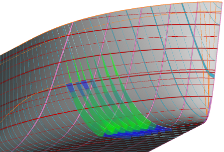
If switched on, curvature plots also show on selected polycurves. If a set of consecutive polycurves is selected in parallel planes, which is easiest done from the tree view, a plot appears on each of them. This visualises curvature transitions across curves, which can be a valuable insight. You way want to enable colour coding of the curvature plot, so overlapping plots can still be read, using [File]→[Preferences...]→[Curves]→[Curvature].
At SARC we have a focus on keeping mouse travel distances low, and the previous Fairway GUI was known for its keyboard shortcuts and the swift operation they allowed. Even though the current GUI has more buttons and dials than its predecessor, we have maintained our commitment and the keyboard is still a fully supported control device.
The menu bar is activated through the <Alt> key like you are used to, after which mnemonics are displayed for the keys that activate the menu items. Some items like [File]→[Save], [Undo]→[Undo] and [Undo]→[Redo] can be activated without opening the menu, by pressing the shortcut key combination that is displayed to the right of the item in the menu.
As discussed in Modelling actions, many modelling actions bring up a dedicated panel with relevant controls and information. This action panel stands out visually with a distinct background colour, so it is easily located on the screen. Most controls on the action panel have a corresponding item in the context menu, which can be brought up with a click on the right mouse button in a modelling view. Whenever the context menu is up, hotkeys are displayed over the controls on the action panel, so they are easily memorised while using the program. These keys are “hot” whenever the control is visible, unless an input field has keyboard focus. Pressing a hotkey simulates activation of the associated control on the action panel.
Fields for numerical input always show the unit of the number, unless it is dimensionless. If digits are selected in the field, then these are replaced instantly upon the first key-press. Double-clicking selects the digits before or after the decimal mark, and a third click selects the entire number.
Often, real numbers are displayed in reduced precision to save space on screen, but when they are being edited the field may expand to reveal more digits. This allows the number to be inspected and edited at a higher precision.
If small arrow buttons are shown next to the field then these may be clicked (and held) to change the value in predefined small steps. The same can be accomplished by pressing the <Up> and <Down> arrow keys. Bigger steps are made with the <Page Up> and <Page Down> keys. A third way of adjusting numbers is by rolling the mouse wheel over an input field. If you do that while holding the <Ctrl> key, then bigger steps are used. For this it is not necessary to click on the field first, it suffices to place the mouse pointer over the field and start rolling.
Read on to learn about Navigation.