|
PIAS Manual
2026
Program for the Integral Approach of Shipdesign
|
|
PIAS Manual
2026
Program for the Integral Approach of Shipdesign
|
This action is at the core of Fairway modelling, and packed with functionality. It is started from [Curves]→[Change the shape of the curve] (keys <Alt><C><S>), or by selecting a curve and clicking on one of its points or vertices, or from the context menu after clicking the right mouse button on a curve in the tree view.
There are three main ways to change the shape of a curve. Firstly, it is possible to change the points of the curve, and let Fairway fair the curve through the points. Secondly, it is possible to change the curve directly, by changing the vertices of the control polygon or setting the curve type or specifying boundary conditions. The third way is to define a master/slave relation between curves, in which the curve shape is derived from the shape of a master curve.
The action panel provides three tabs to work in either of these three ways: the [Points] (key <P>), [Curve] (key <C>) and [Master] tab (key <M>). The tab in the top right corner of the action panel provides optrefen{fwy_action_curve_shape,fwy_action_curve_shape_settings} with which the behaviour of the action can be adjusted.
Below the tabbed section there are four general purpose buttons: [Fair], [Process All], [Clear] and [Redistribute]. These are discussed below.
When [Process All] is pressed (keys <Shift+P>), all the points of the curve are shifted onto their closest position on the curve, within their freedom of motion. This is an important part of the effort to maintain a consistent network, as defined in the introduction. By default, this task is automated with the option [Points Follow Curve].
When [Fair] is pressed (key <F>), a new curve shape is computed. Unless the curve type in the [Curve] tab is different from [Spline] and/or a master curve is defined in the [Master] tab, the new shape passes closely through the points. Exactly how close can be seen in the [Deviation] column of the coordinate table on the [Points] tab. The accuracy of the fit depends on the [Mean fairing deviation] given underneath (the smaller that value the closer the curve) and whether points have been given a non-neutral weight factor in the [W] column. Larger deviations, as compared to the mean fairing deviation, are given a redish background in the table to allow for a quick optical quality check.
After fairing, the deviations can be eliminated by processing the points, if this isn't done automatically already.
Alternatively, the curve can be fitted exactly through the points (omitting the ones that are marked inactive in the [W] column) by checking the [Interpolate] option. This will also change the text on the [Fair] button. Care should be taken in using this option, because an interpolating curve may easily oscillate between points if one of them is slightly misplaced, and inflections can spread like ripples. The ability to allow for acceptably small deviations between points and curves is actually one of the strengths of Fairway, and helps in producing fair lines for production.
By default, fairing (or interpolation) is done instantly and automatically with the option [Curve Follows Points] whenever that is appropriate. Nevertheless, that option does not make this button obsolete, as you will see below.
Fairing, in the naval architectural sense of smoothing up and working out unwanted inflections, can often be accomplished by alternatingly pressing [Fair] and [Process All]. Because [Fair] allows for small deviations and [Process All] eliminates them, both curve and points subtly converge to a higher fairness with each iteration. Obviously, if [Points Follow Curve] is on, points are processed immediately, and just pressing <F> a few times will quickly improve the fairness. This can easily be visualised by the curvature plot. The rate of convergence may be increased by increasing the [Mean fairing deviation], but when done it is wise to reset that to the default value by means of the red arrow button behind the input field, as defined in [General Fairway settings].
Because crossing curves are connected through their shared intersection points, fairing one curve may reduce the fairness of other curves. It is easy to switch to a crossing curve and repeat the process there: crossing curves are listed by the coloured buttons in the [Intersections] column of the coordinate table, and pressing one of these will implicitly apply the changes to the current curve and start manipulation of the crossing curve. By repeatedly visiting and fairing the curves in a problematic area, imperfections can be eliminated, producing a fair and consistent network of curves.
Another way to switch to another curve is by selecting a curve from the Tree view, which will also implicitly apply changes to the current curve.
Pressing [Clear] (keys <Shift+Delete>) removes any and all internal points from the current curve. Of course the intersection points with other curves remain.
When [Redistribute] is pressed (keys <Shift+R>), two things happen. First the internal points are removed, like [Clear], and then new internal points are inserted, based on the vertex locations of the spline control polygon. This is mainly useful after vertex manipulation, to help fixate the curve shape during future curve fairings. You may want to [Fair] the curve after redistributing points to verify that the shape is fixated properly.
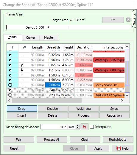
The coordinate table forms a central part of the [Points] tab. It lists all points of the entire polycurve. The subdivision into individual curves is seen in the first column [T] (for “Type”) which differentiates knuckle points from ordinary points. The background of points on the current curve in that column are filled with the colour associated with the curve type. Rows for other curves are marked with a dotted background to indicate that these are not directly manipulated. If there are more points than fit in the table, a scroll bar appears on the right with horizontal marks to indicate the location of knuckles. The current curve is marked with a vertical line on the scroll bar. The cells in the coordinate table can be edited much like a spreadsheet. If cells are edited outside the current curve, changes to the current curve are applied and a new session is started on the other curve.
Cells and columns can be selected with the mouse, and the key combination <Ctrl+C> copies the selected values to the system clipboard, much like a spreadsheet does. In the same manner, values from the clipboard can be pasted into selected cells of the coordinate table with the key combination <Ctrl+V>. Only editable cells of the current polycurve segment will be overwritten.
Directly underneath the coordinate table are the mode buttons, from which there is always one depressed: [Drag], [Knuckle], [Insert], [Delete], [Weighting], [Swap], [Process] and [Reposition]. The mode determines how the mouse works in the modelling view.
The [Drag] mode (key <D>) on the [Points] tab simply allows for interactive manipulation of the positions of points by means of a dragger, introduced in The dragger: interactive graphical positioning. If [Curve Follows Points] is on, dragging points is an effective tool for manipulating the shape of the curve.
If the position of a particular point needs to be keyed in exactly, make sure the dragger is snapped onto that point and press <F2>. This will teleport the mouse pointer over to the corresponding row in the coordinate table and open the first editable cell for editing. You may switch between cells with <Tab> and <Shift+Tab>. See also Numerical input.
The [Knuckle] mode (key <K>) lets you toggle the type of a point between knuckle and ordinary. This effectively splits or joins curves in the polycurve. Because the [Change the shape of a curve] action can only work on one curve at a time, any changes to the current curve are applied right before a knuckle is toggled on or off. The point nearest to the mouse pointer will light up and a message in the status bar shows what will happen to it if the left mouse button is clicked.
It is also possible to toggle knuckles in the left-most column of the coordinate table by means of a double click, <F2> or <Space>.
The [Insert] mode (key <I>) on the [Points] tab simply allows you to insert extra internal points on the curve. The position at which the point will be inserted is shown dynamically in the prelight colour, and you can preview its exact coordinates on a temporary row in the coordinate table. Click to insert a point.
The [Delete] mode (key <Delete>) on the [Points] tab is for deleting internal points on the curve. If a certain point cannot be deleted, the reason why is displayed on the status bar.
In the [Weighting] mode (key <W>), the relative importance of points can be changed between neutral, inactive and heavy. Instructions on how to do that appear in the status bar. An inactive point is marked with an outlined arrow pointing upwards, a point with a heavy weight is marked with a filled arrow pointing downwards.
As with knuckles, it is also possible to change weights in the [W] column of the coordinate table by means of a double click, <F2> or <Space>.
In the figure below a situation is sketched in which it may be necessary to swap two points on the curve.

On the left a frame is shown with points numbered in sequence. Points 3 and 4 mark the intersection with a waterline and buttock respectively. Together the three curves form the sides of a triangular face. Then a manipulation is performed (middle figure) that causes the frame to pass the intersection between waterline and buttock on the other side. Geometrically the triangle has been flipped (look at its corners) but the connections remain unchanged, so in effect the triangle is oriented inside-out: Points 3 and 4 remain on their respective curves, so now the points are ordered out of sequence, producing a kink in the curves. By swapping points 3 and 4 the order can be restored and the kinks untangled (right figure).
The [Swap] mode is designed to swap the corners of a triangle, flipping it topologically. The following requirements and limitations apply:
Any pair of points nearest to the mouse pointer that satisfy this requirement will light up, and be swapped upon a click of the mouse.
Sequencing problems around faces with a higher number of sides or of a higher complexity than the above cannot easily be repaired. Often the fastest solution is to delete the problematic polycurve entirely and reinsert it. Another solution is to split it up, remove the kink and reconstruct the missing part by connecting points. See Split polycurve, Remove Polycurve and Connect Points.
In the [Process] mode, individual points can be shifted onto the curve, within their freedom of motion.
In the [Reposition] mode, individual points may be shifted along the curve, if their freedom of motion allows this. If not, an explanation will appear in the status bar. Care should be taken not to shift points past neighbouring points, which would bring them out of sequence, causing a kink in the curve when it is faired.
The [Curve] tab is divided into two sections. In the upper section, the curve type can be specified, which also enables controls that are relevant to the type. In the lower section, boundary conditions can be set and manipulated to the start and end points of the spline.
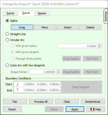
As explained in Lines, a spline is a freely malleable curve, both by vertex manipulation and by the fairing algorithm. All other curve types produce a fixed shape. The default colour associated with splines is light blue. Splines may have specified boundary conditions at both ends. There are four modes for vertex manipulation.
In the [Drag] mode on the [Curve] tab vertices can be moved by means of a dragger. It is often easier to design good curves with a low number of vertices, therefore you may want to [Delete] vertices first.
In the [More] mode on the [Curve] tab, more vertices may be added locally to give more shape control. Existing vertices will be shifted to preserve the current shape of the curve. Highlighted vertices will be shown to indicate where vertices will be positioned if the mouse button is pressed.
In the [Insert] mode on the [Curve] tab, additional vertices may be inserted into the control polygon. This will change the shape of the curve. It is possible to quickly “sketch” a shape with a string of vertices by giving a sequence of clicks in the graphical view.
The [Delete] mode on the [Curve] tab simply allows vertices to be deleted from the control polygon.
Straight lines remain straight and are unaffected by fairing operations. Curves in flat sections of the shell can advantageously be defined as straight lines. When a curve is turned into a straight line, any existing boundary conditions are removed. The colour associated with straight lines is green by default.
The default colour for circular arcs is light grey. Arcs with a given radius can only exist in polycurves that are defined in a plane, not in spatial polycurves. The arc can be flipped to the other side by inverting the sign of the radius.
Arcs with a given tangent have always one tangent defined. The tangent can be changed in the lower section of the [Curve] tab. You are free to define a tangent at the other end, which will remove the existing boundary condition.
This type enables two modes. The [Drag Position] mode displays a dragger with which an arbitrary position can be set that the arc will pass through. Using the [Pick Point] mode the arc can be made to pass through an existing point on the curve.
Straight lines and circles are conic sections as well, but this type allows the remaining conic sections to be defined: parabolic, hyperbolic and elliptical arcs. These are defined by a two-edged control polygon, the middle vertex of which is given by the intersection of the two tangents. Consequently, the tangents should be coplanar; if they are not, the curve will find a plane in the middle, but not adhere to the given tangents strictly.
The type of conic section depends on the [Shape Factor]: a higher shape factor will pull the curve tighter to the middle vertex, a factor of 0 will give a straight line. A parabolic is produced with a factor 1, higher factors produce a hyperbolic and lower factors an elliptical arc.
The shape factor can also be determined automatically by specifying a third point that the arc should pass through, analogous to [Circular Arc through three points].
In the lower section of the [Curve] tab there is a table listing the boundary conditions at the start and end of the current curve (for an explanation of curve direction see Lines). In the left column an icon indicates the current condition at each end, as follows:

| No boundary conditions |

| Manually specified tangent |

| Tangent derived from adjacent curve |

| Manually specified tangent, straight end |

| Tangent derived from adjacent curve, straight end |

| Tangent and curvature derived from adjacent curve |
The condition can be changed with a double click on the icon, which brings up a pull-down menu with available conditions. Not all conditions may be available, for instance if there is no adjacent curve at that end. If so, the reason will be given in a tool-tip when the mouse pointer is kept still for a few seconds.
Next to the icons are the coordinates of the current tangent vector. These can be edited in the table or manipulated interactively in the [Drag Tangent] mode, activated with the corresponding button in the table.
On the [Master] tab a master/slave relation can be defined, in which the shape of the current curve, the slave, can be made dependent on another curve in the model, the master curve. Whenever the master curve changes, the slave curve will change also, according to the defined dependency. This is exemplified at the end of this section with the construction of deck camber and sheer strake. A cascade of depedencies can exist, as master curves themselves can be a slave of other master curves, and several curves can depend on the same master curve.
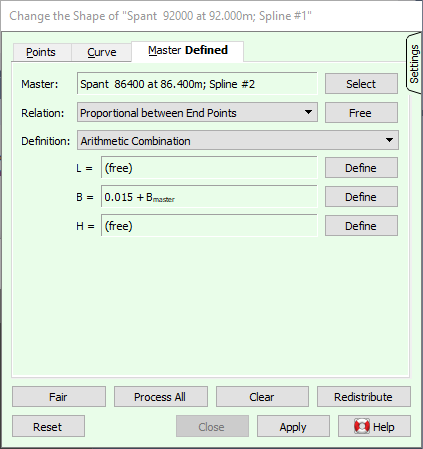
The first step in establishing a master/slave relation is to select the master curve, using the [Select] button. You are free to select a master from any active solid; solids can be toggled active/inactive in the [Access] column of the [tree view] before starting the selection.
An existing relation can be annulled with the [Free] button.
Next steps are to select the proper relation and the definition of the dependency.
The relation defines how points on the current curve are mapped to points on the master curve and vice versa. Choose between these four relations:
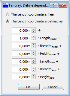
The last step in the configuration of a master/slave relation is how points on the current curve are defined, based on points on the master curve.
The current curve will be shaped similary to the master curve, offset from the master curve in a direction and distance that may vary over the length of the curve. The direction is perpendicular to the projection of the master curve onto a certain projection plane. This plane can be visualized by pressing the [Drag Plane] button, which will also reveal a rotational dragger with which the orientation of the plane can be manipulated interactively. You may also key in the components of the vector manually, and the plane can be made to fit the master curve using [Master Plane], or the offset can be defined in the current view-plane of the active camera by pressing [View-Plane].
The offset distance can be specified for the start and end point individually, which will produce a linear transition over the length of the curve. These can also be dragged interactively using the [Drag Offset] mode, which will show a linear dragger snapped to the curve end nearest to the mouse pointer.
Let's say you want to construct a deck with constant camber of 2/100 of the local breadth of the deck. To do that we start manipulating the deck profile line at the plane of symmetry. Then we select the deck line in the side as the master curve, whose transverse coordinates mark half the local breadth. We will set the relation to [Longitudinal Position], because both curves generally run longitudinaly. We want breadth to be unaffected (free) as well as length, but the height should equal the height of the deck in the side plus 4/100 of its breadth. So we define an arithmetic combination of \(H = 0.04 \cdot B_{master} + H_{master}\).
If you need to construct a sheer strake then this is one way to do it: Start manipulating the curve that marks the lower seam of the sheer strake and select the upper seam as master curve. The relation can be set to ‘Proportional between End Points’ or ‘Longitudinal Position’; which is the better option depends on the hull shape and you may try both to select the appropriate one.
Now set the definition to ‘Offset’, and define an offset plane parallel to the center plane, with normal (0.0, 1.0, 0.0). Finally the height of the sheer strake can be specified at the front and end of the seam.
This produces a sheer strake of constant width as seen from the side.
The [Settings] tab in the upper right corner of the action panel automatically expands if the mouse pointer is moved over it. This tab contains some options with which the behaviour of the action can be adjusted.
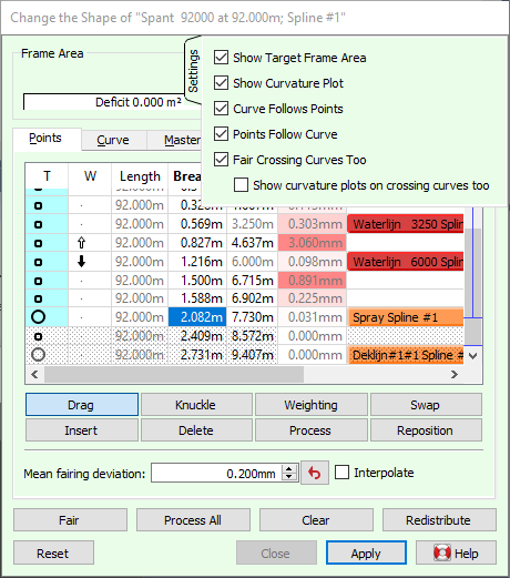
If a target sectional area curve (target SAC) has been constructed, see Change the shape of the SAC, you may want to compare the current frame area (below the construction waterline) with the corresponding point on the target SAC. The option [Show Target Frame Area] toggles an additional [Frame Area] section at the top of the action panel, as shown above; provided the current curve is part of a frame. It can be removed at any time with the cross button in the top right.
Shown is the target area according to the SAC, and a bar graph indicating the surplus or deficit area of the current frame, as compared to the target. The [Fit] button will transform the current frame so that its area matches the target SAC, while its shape will be preserved as much as possible. Further details are found in Hullform transformation. If no target area is available, then probably no target SAC was generated, or it does not extend to the current frame position.
Together with the [Frame Area] section in the action panel, appears in the moddeling views a transparent rectangular plane. The area of this plane equals the target frame area, while the height is equal to the design depth. This may help optically in designing the frame shape, as the area under the frame within the rectangle needs to match the area from the frame up to the construction waterline outside the rectangle.
With the [Show Curvature Plot] option on the [Settings] tab the curvature plot can be switched on during curve manipulation, even if curvature plots have been switched off in general; see Prelit polycurves. The plot is also shown for any curves in the polycurve that are directly preceding or succeeding the curve under manipulation, as these may change shape when their common knuckle point is dragged or when they follow a boundary condition with the current curve.
For reasons of consistency this option is automatically switched on when the general curvature plot is on or is being switched on. Conversely, the general plot is automatically switched off when this option is being unchecked.
If the option [Curve Follows Points] is checked, then the curve is instantly and automatically faired upon any change in the information on which the fairing is based. Most notably, when this is on, the curve can be interactively shaped by dragging points and tangents. In many cases this can be an effective alternative to shaping the spline through its vertices, and has the added bonus that the shape remains fixed during future curve fairings. For vertex manipulation, on the contrary, generally requires the shape to be explicitly fixated, which still is no quarantee against subtle changes during future curve fairings.
If the option [Points Follow Curve] is checked, then all points will be processed automatically (shifted onto the curve) whenever the shape of the curve changes. Together with [Fair Crossing Curves Too] this is a great help in keeping the network consistent at all times.
If you switch this off, you will most probaly want to [Process] individual points or [Process All] before you apply the shape changes.
Check this if you like all curves that pass through the points of the current curve to adapt dynamically to any changes in their position. This is a great help in keeping the network consistent.