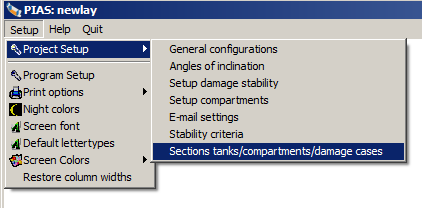
With this module the choices and parameters for calculations, calculation variants and output can be set. This module can be activated as independent PIAS module from PIAS&apos main menu, although most options are also available through the Project setup function, at the left-hand side in the upper (menu) bar of each other PIAS module, as depicted below.
Project setup function in each PIAS module.
In this module general program settings can be defined. These are not:
Defined here are program settings — occasionally a computation method — which are applicable to more than one single module.Config starts by showing its main menu, which contains the distinct setup categories:
Calculation methods and output preferences
At this option the desired output format can be selected, such as output language and file format, as well as some general settings which are applicable to the hydrostatic calculations, such as calculation methods, wave particulars and the density of sea water.
Output language
Here the language can be specified as used for the output of calculations and the like. Choices are e.g. Dutch, English, German and Chinese, but only the first two are available in all PIAS modules. If a language is selected that is not available in a particular module or output, then by default English will be used. Incidentally, each user is able to expand the supported languages, see Output in different languages.
- Attention
- If the output contains a row of question marks instead of plain text, then PIAS has encountered an unavailable translation. In the link stated just above the procedure to handle such anomalies is discussed.
Apply Local cloud
With this option set to ‘yes’ for this project the local cloud, a concept which is discussed at Local cloud: simultaneous multi-module operation on the same project, will be activated. However, for the time being this option is still experimental, so it is not yet released for general use.
The module Loading always prints an item in the loading conditions which represents the total light ship weight. This total weight represents the combined weight of items from the ‘common list&rsqauo. The name of thislight ship weight can be specified here.
Stability calculation method
With this setting the calculation method of intact and damage stability can be chosen, with a choice from four options:
- With fixed trim. At zero inclination the ship has its initial trim, depending on the difference between LCB and LCG. This trim is kept constant for all angles of inclination, and used during the computation of stability. This ‘fixed trim’ option is applicable to intact stability.
- With free-to-trim effect (=constant LCB). Also, in this case the ship has its initial trim. When the vessel heels for each heeling angle the real trim is calculated so that the longitudinal center of gravity coincides with the longitudinal center of buoyancy. This is also known as then ‘constant LCB method’. It will be obvious that in general the trims will be larger with a vessel of a longitudinally asymmetric nature, such as a supply vessel at larger heeling angles.
- With free-to-trim effect, including the effect of VCG on trim. With only ‘free-to-trim’, when calculating intact or damaged stability, PIAS determines longitudinal equilibrium (and consequently trim) by coinciding longitudinal center of buoyancy with the longitudinal center of gravity, which means that they are on the same longitudinal location. The implicit assumption behind this method is that the forces act perpendicular to the base line (which is the longitudinal axis), however, with a trimmed vessel this is obviously not the case. This simplification results in a small trim inaccuracy, which is larger at larger trims and higher VCGs, but which is sufficiently small in normal cases. However, it might be desirable to make a somewhat more accurate computation by taking the forces perpendicular on the waterline, which is done with this setting at ‘yes’. With this setting one should also realize the other effects, such as:
- Stability calculation results do not necessarily have to agree with results of computations based on tables of maximum allowable VCG', because there the effect of VCG' on trim is not included (which would be a bit difficult to do, because the actual VCG' of the loading condition was unknown on forehand, when composing the VCG' tables.
- Stability calculation results might differ from manual calculations as composed with the aid of cross curves, because it would not be possible to compose them for the actual VCG' of the loading condition, as well as for all other VCGs of all other loading conditions. In theory multiple cross curves for multiple trims could be composed, but nobody does and nobody requires so.
- Heeling around the weakest axis. With the previous three methods, heeling occurs around, more or less, the longitudinal axis of the vessel. With this method automatically the axis of weakest stability is determined. Therefore, this method is the most realistic of the four. This setting is only implemented in PIAS in calculations where it is relevant and consistent, so e.g. for the calculations of intact and damage stability, but not for e.g. cross curves and maximum allowable grain moments. The background of this method is described in a separate document Stability around the weakest axis in PIAS; explanatory notes, which is available at SARC on request.
(Damage-) stability including the shift of COGs of liquid
The conventional way to take free surfaces into account is by correcting the vertical center of gravity by a virtual increase due to the free surface(s) at heeling angle zero. This virtual increase of the actual VCG is taken constant at all heeling angles. However, in reality the free surface effects change due to heel and trim.
- If this option is answered with ‘No’, the (damage-) stability is calculated in the traditional way with a VCG correction which is constant for all heeling angles.
- If this option is set to ‘Yes’, and if this option has been purchased, then for every compartment containing a liquid the actual center of gravity is calculated at the actual heeling angle and trim at the intact stability and damage stability calculations (with the Loading module).
This option set to ‘Yes’ has the following consequences:
- Tables of maximum allowable VCG' are no longer valid while the virtual center of gravity G' has become meaningless.
- Centers of gravity and free surface moments printed in loading conditions may differ from the input data. Due to heel and trim the centers of gravity may have shifted and the surface of the liquid may have a different shape than at zero heel and trim.
- All weight items (in Loading) which contain liquid cargo should be of types ‘tank’ or ‘floodable tank’. Weight items from different types which yet have a non-zero value for Free Surafce Moment are not allowed.
Preferential format of hull files
PIAS can perform hydrostatic calculations and (damage) stability calculations on the basis of two of the representations as discussed in Hull form representations :
- The frame model, which essentially consists of cross sections (ordinates), and which may be defined by Hulldef or generated by Fairway.
- The triangulated surface model, which is essentially a representation of the hull surface (including differentiating inside and outside), which can be produced by Fairway.
In principle, a surface model can be more precise, particularly when determining the shape of small compartments. However, it has a major objection, and that is that, in order to be sufficiently precise, the number of triangles of the hull surface must be rather large, leading to correspondingly long computation time. Therefore, in practice, the surface model is not used for ordinary calculations. PIAS also has a third option, which is ‘calculate with frame model, plot surface model’, with which all calculations are based on the frames, while in the graphical presentation — e.g. as in the GUI of Loading — the full surface model of the hull is shown. That setting offers a nice compromise.
Density outside water
Enter here the density (the specific weight of the outside water (sea water, in ton/m3) to apply for all hydrostatic, stability etc. computations. As a rule, for sea water 1.025 is taken.
Calculate intact stability etc. with a heeling to
For the sake of all stability-related calculations, angles of inclination can be given (see Angles of inclination for stability calculations). That leaves the question of which side (PS, SB or both) these angles should be applied. Which is controlled here, by a choice from four options:
- Portside.
- Starboard.
- The side of the heel. With this setting, the side of the worst stability is estimated with this method: if the statical angle of inclination (the heel) is to PS then the calculation is made to PS, otherwise to SB. With zero heel the calculation is (therefore) to SB. This estimation will often be correct — in the sense that that is indeed the side of worst stability — and sometimes not; e.g. when the heel is to SB, but openings on PS are submerged at a much smaller angle than on SB. If one does not want to rely on an estimation in determining the side of worst stability than the fourth option can be used.
- Portside and starboard. With this setting there will be no a priori assumption on the “worst side”, instead the stability will be calculated to PS as well as SB, while both sides are fully taken into account in the stability assessment. If stability criteria have been defined (and selected, see Manipulating and selecting sets of stability criteria) then also a maximum allowable VCG' can be determined, which will be the minimum of all stability criteria and both sides.
The third option is the default, but that does not mean that the user should not rethink the applicable choice for the vessel under consideration. In any case, one must realize that the more asymmetrical the ship is (in terms of hull shape, openings or compartments) the less accurate the first three options can be. Obviously, the fourth option will require more computations, and hence more calculation time.
Please take in this respect also take note of the opening remark of Types of basic criteria.
Calculate damage stability with a heeling to
This option is similar to the previous, albeit applicable for damage stability instead of intact stability.
Backward compatibility in calculations
Rarely, one of the central computation algorithms from PIAS is modified. If feasible in such a case, a switch may then be added which makes the program still to apply the original algorithm. In general, it is discouraged to use such a backward compatibility mode, because the whole reason for the modification will be that the new algorithm will be better (e.g. faster, more accurate or more robust) than the original. However, if you need results to be compatible with previous PIAS versions — for example for existing designs or elder projects — you can set that here. This option is only available in Config, not from the Project setup in the menu bar of other modules. At present only a single switch exists, namely:
Volumetric computations with the method from before December 2016
For the implementation of octothreading, in December 2016 some core volumetric integration procedures of PIAS have been redesigned. In that process the accuracy of one particular algorithm was increased a bit. That algorithm existed for more than 25 years, but the steadily increased computer power allowed a refinement to be incorporated now. Due to this modification, hydrostatics and stability-related results of PIAS might differ from earlier versions. If this box in the popup window is ticked on, the pre-December 2016 algorithm will remain to be used for this project.
Output filetype
If the output has been redirected to File, see Print options, then a file will be generated of the selected output filetype and with the file name as given on the next line. Supported file formats are (please also refer to the somewhat more detailed discussion in Export of results):
- ASCII. With this option only alphanumerical output (tables and text) are send to file, graphics, layout and formatting are lost.
- Rich Text Format. Contains the complete output, including all formatting and graphs, in RTF, which can be imported into a word processor such as MS-Word or OpenOffice.
- Drawing Exchange Format (DXF). Drawings and graphs are stored in a file according to the Autodesk DXF specification, which can be imported into e.g. AutoCAD or Rhino.
- Postscript, which will save drawings in vector format. This has the advantage of being resolution-independent, which results in much more sharpness in large or highly zoomed drawings.
Angles of inclination for stability calculations
With this option the angles of inclination which will be used at the intact and damage stability calculations can be defined, with a maximum of 100. The angles may be larger than 90°, however, not larger than 180°. Angles between 85° and 95° are not allowed. On the angles as givenhere two expections may be applicable:
- For probabilistic damage stability calculations it can be set that PIAS should use a default setting for angles of inclination, as discussed in Compute probabilistic damage stability on basis of.
- Using Consecutive Flooding, trough pipe connections and internal flow over thresholds, discontinuities may occur in the stability curve. In order to model these neatly, with such calculations internally many more angles will be used, as described in Basis of larger angle stability (GZ-curve).
Settings for compartments and tank sounding tables
This menu contains settings which are applicable to tanks and compartments:
- Tables with everywhere the maximum free surface moment. By default, the free surface moments as printed in the tank tables are for the actual filling level of the tank. If this option is set to ‘yes’, then first the maximum free surface moments will be computed for the present tank, after which for each height (in between completely filled and completely empty) instead of the actual moments these maximums will be inserted. After toggling this setting, the tank tables in Layout should be recalculated before this setting exerts its effect. Moreover, any previously calculated table should be discarded first.
- Difference internal/external geometry including external hullforms. This setting is applicable to the comparison of internal and external geometry, such as has been discussed in Difference between internal and external geometry. If set to ‘no’ this comparison does not include added hull forms (as discussed in Hullforms. If set to ‘yes’ it does take such hull forms into account.
- Direct calculation of tank data. If this option is selected, the tank data in the loading conditions is no longer determined by interpolation on the pre-calculated tank tables, but by a direct calculation of the current volume or liquid level. The tank data is also calculated immediately when the tank tables are printed in the Layout module. There are no pre-calculated tables available in Layout. The tables can be checked by printing them.
General settings damage stability
Calculation damage stability according to the method of
On this line, one can specify which method should be used for compartment connections and (internal) openings and so on. Two systems exist for this purpose, viz. ‘Complex stages’ and ‘Consecutive Flooding’. The first has been in development from ±1990 to 2022, supporting virtual connections between compartments, including so-called ‘critical points’ with which thresholds and internal openings can be modelled. The second is available from 2023, and supports the entire topology and geometry of internal connections, pipelines, valves, check valves etc. Both systems are discussed in extenso in Background from tools for ship-internal connections in PIAS.
To be elaborated: include the list as present in the Dutch manual version.
Calculation Consecutive Flooding according
Consecutive Flooding currently has two variants to choose between here:
Time domain calculation time step
As explained in Damage stability in time domain, this method essentially simulates the continuous flooding process with a series of very small steps in time. The duration of such a step, in seconds, is specified here. Incidentally, this is a global setting belonging to the vessel as such. At the detail level a more specific time step can be specified, see the discussion at Properties of piping networks. Todo: and in Loading.
Time domain maximum number of time steps
The previous setting manages the calculation process, but carries the risk that using a time step that is (in hindsight) too short will result in extreme computation times, and corresponding output. To limit this, the number of time steps can be capped here. Please also consult the discussion at Basis of damage stability in time domain.
GZ calculation interval in seconds
At each time step of a time domain calculation, fluid flow, draft, trim and heel will be calculated. In addition the full stability (a GZ curve over all heeling angles) could also be calculated. However, if that is done for each time step it could lead to a large amount of output that is by no means all relevant.
To mitigate that, this setting, together with the next, manages on which steps a full stability calculation will be made. For example, if 15 is specified here, then every 15th step the GZ will be calculated (and verified against the stability criteria). Incidentally, around the first and last time steps the GZ will always be calculated, because that is supposed to be interesting anyhow, regardsless of the setting here.
Minimum weight difference for a GZ calculation
This setting pairs with the previous. At the beginning of a time-domain process, in general the fluid flows are quite strong, but towards the end they become less and less so. This means that the differences per time step towards the end are also small, so that even when limiting stability output using the previous parameter still quite a lot of, not always relevant, output may be produced. One can further reduce that additionally with this parameter; here one specifies what the minimum difference in total weight (in ton) with the previous full stability calculation should be. So if you enter 22.45 here, the stability is only calculated at that step where at least 22.45 ton of fluid has been displaced with respect to the previous full stability calculation.
Maximum allowable equalization time
For the purpose of time-domain calculations: the maximum time for the ship to come to rest, after damage and water ingress. This paremeter is used to determine in which cases final-stage stability criteria are applied, and when those for intermediate stages, see discussion in Choice of stability criteria with the time domain method.
Percentage of transferred liquid at which equalization is considered ready
The whole idea of a time domain calculation is to calculate the time in which the fluids equalizes. That is finished when the whole system of vessel and fluids have come to rest. However, towards the end of the process the fluids start to flow slower and slower; after all, the level differences get smaller, and hence the pressures, and hence, courtesy of Bernoulli, the flow velocities and flow rates. In essence, it is an asymptotical process where after, so to speak, many hours, milliliters are still flowing through the pipelines and openings. Indeed, in theory, equalization time will always be infinite. In practice, there is a certain tolerance in PIAS, so that if e.g. the difference in draftt between two consecutive time steps is less than a mm or 1/10 mm that is considered as ‘rest’. However, that is an arbitrary tolerance that unintentionally has a large outcome on the final answer; at 1/10 mm, the equalisation time can easily be twice as long as at 1 mm.
One might think of implementing in a practical limit; after all, we are interested in the tons flowing through the system in the early time, and not so much in the millilitres in the last seconds. With that idea, a criterion can be formulated that is related to the transferred weight. For example ‘if 98% of the total, final, fluid weight has flown through then I consider the system at rest’. The default percentage used in PIAS is indeed 98%, but this Config setting allows the users to adjust it as they see fit. The effect of this setting is visualized in the figure below.
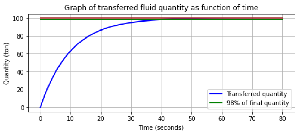
Transferred liquid as function of time.
Minimum sectional area for instantaneous fluid passage
If the cross-sectional area of a pipe or connection is larger than the area specified here (in m²) then the water will flow freely through it during heel, and otherwise not. Background to this is discussed in Basis of larger angle stability (GZ-curve).
- Attention
- Please acknowledge that the minimum area is given here in m2, while pipe' cross-sectional areas in Layout ar egiven in cm2.
Permeability of connected compartments
The good old art of naval architecture has brought our community differences in permeabilities (μ) to be applied, e.g. 98% for an intact compartment and 95% when it is damaged. For the same compartment! Although this convention is nonsensical, PIAS is adapted to it anyway, given e.g.&the different types of μs that can be assigned to each compartment, see Permeabilities. However, that is not the end of the story, take for example:
- A damaged compartment, connected to another non-damaged space, by a tiny water pipe. This other space ‘feels’ somehow intact, so should the intact μ then consequently be applied?
- The same damaged compartent, now connected to another space by a large duct. This ‘feels’ like being part of one global damaged space, so the damaged μ should now be applied? Or not? This configuration is in principle not different than the previous.
So, there is no intrinsic logic which guides us here. But perhaps the regulations provide a clue? Let's have a look at two of those:
- SOLAS 2020, chapter II-1, part B (probabilistic damage stability) reg. 7-3: “For the purpose of subdivision and damage stability calculation of the regulations, the μ of each compartment shall be as follows: (followed by a table of damaged μs)”. This line implies that the damaged μs are applicable to all compartments, so the damaged as well as the connected (i.e. flooded but not damaged) compartments.
- IBC Code 2016, §2.7.2: “The permeabilities of spaces assumed to be damaged shall be as follows: (followed by a table of damaged μs)”. This implies that the μs stated here are applicable only to the damaged comps, so connected non-damaged compartments should be assigned a μ as used for intact condition.
More rules could be investigated, however, to cover these two opposite expressions will already require a PIAS setting, which regulates the μ to be used for non-damaged, connected compartments. Because a user will choose this setting based upon the applicable regulation, this single global setting will suffice. With the choice between ‘Use tank permeability’ and ‘Use permeability damaged’
- Attention
- Please do realize that when selecting ‘Use tank permeability’ for all potentially connected compartments in Layout a realistic value for ‘permeability as tank’ must be specified, also for the dry compartments. The default of 98% for e.g. an engine room will probably not be considered realistic.....
Righting levers denominator
Stability standards are in general related to righting levers, and derived parameters such as GM and area under the righting lever curve. However, in the essence, during a stability calculation righting (and heeling) moments are computed, instead of levers. Converting from moments (ton.meter) to levers (meter) is conveniently done by dividing by the vessel's displacement. For intact stability this displacement (the denominator in the division) is unambiguously the one and only factual displacement for the particular loading condition. However, for damage stability choosing the denominator is not that obvious, should for example the displacement be corrected for the liquid cargo loss, and/or the weight of the ingressed sea water? The relevant regulations provide two alternatives for this choice, which have both been implemented in PIAS:
- Constant displacement. With this setting the denominator is simply the intact displacement. This is the conventional choice, e.g. applicable to:
- Code for the construction and equipment of ships carrying dangerous chemicals in bulk (1980 edition), guideline for the uniform interpretation, reg. 3.2: “The GM, GZ and KG for judging the final survival conditions should be calculated by the constant displacement method”.
- MSC.1/Circ.1461, Guidelines for verification of damage stability requirements for tankers (applicable to IGC and IBC 2016), reg. 3.3.3, as well as IACS 110 Guideline for Scope of Damage Stability Verification on new oil tankers, chemical tankers and gas carriers (2010), reg. 3.3: “When determining the righting lever (GZ) of the residual stability curve, the constant displacement method of calculation should be used”.
- SOLAS 2009 probabilistic damage stability (part B.1), reg. 3 “When determining the positive righting lever (GZ) of the residual stability curve, the displacement used should be that of the intact condition. That is, the constant displacement method of calculation should be used”.
Before PIAS was extended with this setting Righting levers denominator (in July 2018) this was the standard choice for the denominator.
- Intact displacement minus liquid cargo loss. This alternative is offered by MSC.1/Circ.1461, guidelines for verification of damage stability requirements for tankers (applicable to IGC and IBC 2016), reg. 9.3.4, as well as IACS 110 Guideline for Scope of Damage Stability Verification on new oil tankers, chemical tankers and gas carriers (2010), reg. 9.3: “Noting that calculation of stability in the final damage condition assumes both the liquid cargo and the buoyancy of the damaged spaces to be lost, it is therefore considered both reasonable and consistent to base the residual GZ curve at each intermediate stage on the intact displacement minus total liquid cargo loss at each stage”.
- Note
- Now and then, this choice of denominator is confused with the methods of lost buoyancy vs. added weight. However, these are distinct concepts: lost buoyancy vs. added weight refers to the iteration method used to find equilibrium between weights and buoyancy. In the pre-computer era this issue carried some relevance because it determined the computational efficiency, but with abundant computer power it has become irrelevant. After all, both methods lead to the same observable parameters (draft and trim) which is quite obvious because otherwise one of the two would be outright false, and could easily be identified as such on the basis of a physical (model) test. Constant displacement vs. Intact displacement minus liquid cargo loss is not a method, it is just a single number to be divided by, which only exerts its influence on the GZ (and hence derived parameters). While GZ is not a primary physical quantity, it is a derived parameter, valid only within a particular reference framework. Apparently, there are at present two of such frameworks around, which may lead to different GZs, without a physically-based referee to judge on their correctness. So, guidance for the denominator to use can only be found in the rule of man-made law (as well as in the stance of consistency).
Intermediate stages with global equal liquid level
This option defines the regime of intermediate stages of flooding. For the damage stability calculation, the vessel is subdivided in multiple compartments, which can be damage simultaneously. For the final stage of flooding the presence of multiple damaged compartments gives no ambiguity, however, with intermediate stages itis the question how the ingressed water is distributed over the compartments. Suppose two tanks become damaged, and the flooding stage is 50%, then there are two options:
- Compartments with an unequal water level. Every compartment has half of its weight in the final stage (the 100% stage of flooding). In this case all tanks are treated separately, the water levels of tanks 1 and 2 differ, and there are two free surface moments. This is depicted in situations 1 and 3 of the figure ‘Tank fillings’.
- All compartments with an equal water level. All damaged compartments combined are half the weight of the total weight in the final stage of flooding. So, all compartments are treated as one with one single water level and a single free surface moment, as depicted in situations 2 and 4 of the figure.
The appropriate choice of the method of calculation depends on the configuration of the compartments which are damaged. If these compartments are separated by vertical bulkheads as in situations 1 and 2 then the first choice would be the most realistic. If, on the other hand, the compartments are separated by horizontal bulkheads as in situations 3 and 4 then the second choice would be the most appropriate.
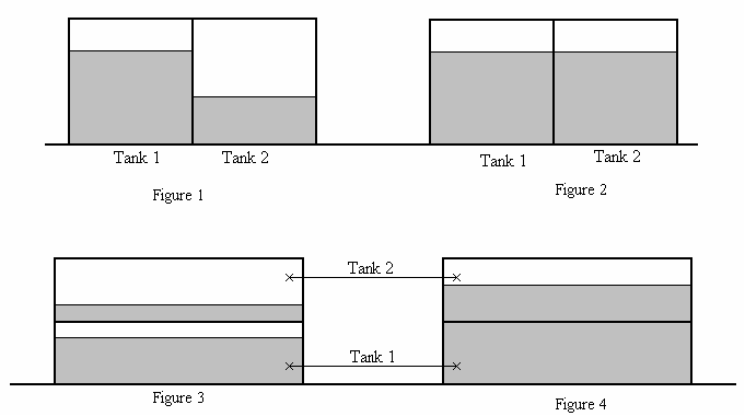
Tank filling
- Attention
- This feature has long been redundant, as the same effect can be achieved with the systems for managing intermediate stages, as discussed in Internal flooding in case of damage, through pipe lines and compartment connections. Therefore, it will be removed from PIAS in the course of 2025.
Compute probabilistic damage stability on basis of
Here it can be set for the computations of probabilistic damage stability, as well as maximum allowable VCG in damaged condition, which angles of inclination to apply:
- User-defined angles. With this choice the angles of inclination as specified at Angles of inclination for stability calculations will be used. The advantage of this setting is that this is the same calculation basis as employed at the Loading module, where the GZ curve is also computed on the specified angles. So, this choice results in the same results for both computations.
- Default angles. With this setting the angles are chosen automatically, guided by the applicable stability criteria. The advantage of this setting is that the user is relieved from choosing the angles, the range for example will always be sufficient to match the stability criteria. The disadvantage may be that these angles may be different from the ones as employed in Loading.
This is, by the way, exactly the same setting as calculate maximum VCG on basis of as discussed in Maximum VCG' intact tables.
Significant wave height for SOLAS STAB90+50 (RoRo)
For RoRo ferries with water on deck (a.k.a. as the ‘Stockholm agreement’ or ‘STAB90+50’) the wave height to be used can be given here. Please also refer to Water on deck.
Damage stability with correction 0.05' x cos(phi)
According to the US DDS-079 damage stability criteria, in the computation of damage stability the transverse center of gravity should be corrected with 0.05 feet x cos(φ). That can be specified here.
Automatic propagation of damage case
When evaluating the damage stability results, it might be concluded that a calculation does not comply with the damage stability criteria because an opening of an intact compartment is submerged. One might wonder what the conclusion would be if the flooding would be extended through that opening. The evaluation of such progressive flooding requires some flooding scenario assumptions, and is in general still uncharted territory. But for one particular case in PIAS a provision has been included, with the following details:
- Works with the stability criterion ‘Distance to special points’ (see Types of basic criteria).
- If a particular damage case does not meet this criterion — because the distance from the waterline to such an opening is less than the minimum required — then the conclusion is drawn “It is yet undetermined whether this damage case complies with the criteria”, and an additional damage case is created where the compartment connected to this opening will also be flooded.
- From these additional damage cases also the intermediate stages of flooding are computed, starting with a filling percentage of 1% for the newly added compartments. This reflects the fact that these are just about to be flooded, but also tests whether the original damage case meets the other stability criteria.
- Since the flooding through such an opening may take a long time, it is not certain that in all cases assessment against the stability criteria for intermediate stages is allowed. Therefore, in this case the criteria for the final stage of flooding are applied.
- This mechanism repeats itself, so, if such a newly generated damage case also does not comply because an other opening has a too small distance to the waterline, then a further additional damage case will be created, etc. etc. Until it is demonstrated that it will comply in this case of progressive flooding (in which case the original damage case complies), or until the ship no longer satisfies another stability criterion (in which case the damage case does not comply).
This facility — which has been discussed and agreed with Lloyd's Register of Shipping in April 2016 — is aimed at inland waterway tankers which must meet the ADN criteria. But anyone with access to this facility is, obviously, free to switch it on in this menu for any application.
Sections tanks/compartments/damage cases
Here the sections and other properties of sketches of compartments and damage cases can be given, details are discussed in Sketches of tanks, compartments and damage cases.
Stability criteria
The stability criteria definition system has so many options and possibilities that a dedicated chapter is included, please refer to Stability criteria for intact stability and damage stability.
Wave settings (for stability)
The hydrostatic and (damage) stability calculations can also be executed for the ship in a static wave (a.k.a. frozen wave). You then specify the wave amplitude, the position of the wave top and the length of the wave, according to the sketch below. The default wave amplitude is zero, then the calculations are made for the ship in calm water. This static wave has its effect on the hydrostatic-related calculations, such as:
- Hydrostatics, cross curves and Bonjean tables.
- Intact stability, and all related computations, such as grain stability.
- Damage stability (where the wave does not extent inside the damaged compartments).
- Longitudinal strength (shear force and bending moments).
The static wave given here has no effect on the seakeeping calculations of Motions, as they do not take a single, static wave into account, but an entire distribution of waves (a wave spectrum) instead.
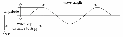
Wave parameters
Wave amplitude
Location of the top of the wave
Wave length
Wave direction
As a rule, a wave as used for the calculation of longitudinal strength or stability is taken to be longitudinally. By exception, it can be required to take an oblique wave, in which case here the angle of the wave direction (in degrees, relative to the centerline) should be specified at this option. Besides, the wave effect in transverse direction is linearized, which implies that the intersection of the ordinates with the wave surface is approximated by a straight line.
Wave type
Two types can be chosen, sinusoidal (the default) or trochoidal.
Settings page heading
This option gives the user the ability to modify the PIAS page heading for all generated output, i.e. to personalize the headings.
- Note
- There are no automatic checks performed to verify if an object is overlapped by another object, but a visual check can be performed using [Print preview].
In this menu you can add and remove page headings and give it an identifiable name. Each new page heading will be the PIAS default. You can select the application of the page heading.
If no page headings are defined or all defined headings are disabled, no page heading appears in the output.
If 1 page heading is defined, and it is not disabled, then it applies to all output pages.
If multiple page headings are defined, then it can be set to use 1 page heading for the first page output and another page heading for all remaining pages output.
Page headings can be exported and imported using their respective options [Export] and [Import] under the option [File], thus a company standard may be defined and exported to be imported elsewhere.
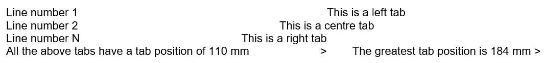
Page heading objects
A page heading is constructed with the help of objects. Each object has to be positioned in with the parameters Line number and Tab position. Different types of objects have different properties. The differences are explained below.
- Object type
- Properties for different types are listed below.
- Normal text
- A user-defined text.
- Title
- The pre-programmed title for that specific output.
- Project name
The project name which is defined in Hulldef or Fairway.
- Date and time
- The date and time when creating the output.
- Date
- The date, without the time, when creating the output.
- Page number
- Start value for page numbering.
- Chapter name
- The chapter name of this generated output.
- PIAS version
- The PIAS version of the program with which the output was generated.
- PC and username
- Which computer and user generated the output.
- Text
- Based on the Object type this column contains a predefined text. The object types that can be defined further are listed below:
- Normal text
Any text which is not covered by a standard type.
- Page number
- The start value for the page numbering. If this text is left undefined then this value should be defined in the popup message when printing. If the W character is present in the text and the copied ‘Rich Text’ output is pasted into a ‘Rich Text’ compatible word processor, then the page numbering is automatically updated to the page numbering of the word processor.
- Chapter name
- Then a popup is posed at the start of a print job, as mentioned in the Page number object, to allow the overriding of the predefined chapter name.
- Font size
The height of a line of text.
- Line number
- The line on which this object has to printed, i.e. the vertical positioning of an object. This is dependent on the text heights.
- Tab type
- The alignment of the object relative to its Tab position, thus a left tab has its alignment to the leftmost part of the object and a right tab to the rightmost part of an object.
- Tab position
- The horizontal position of an object in millimetres.
Overview object positioning
With the option [Print preview] one can check if all objects, in the current page heading, are correctly positioned and not overlapping.
E-mail settings
It is possible to let PIAS send an e-mail after a calculation or print task is finished. The idea is that is sometimes occurs that a computer is busy with a lengthy calculation, and it is inconvenient time after time to look personally whether this task has already finished. In such cases it can be handy if one receives an e-mail, notifying the operator that the job is done. If it concerns a print task with output to RTF file or text file, that file will be send as attachment, so the print results are directly available. This facility has the following settings:
- Send e-mail, with three sub options:
- Never.
- After each print task (and damage stability calculation task).
- After print or calculation of a damage stability module.
- Senders address, recipients address and mail server. As a rule, these will always be the same for a particular computer and user, in which case it is appropriate to set those by means of external variables (see External variables where this mechanism is explained). In other cases, settings in this menu overrule the external variables, and are stored and used per project. So, either nothing is filled in (a blank line), and then the external variable setting will be used, or something is filled in, and then used. By the way, both the computer and the sender must have the right to approach the mail server with e-mail commands according to the SMTP protocol. Furthermore, sending email messages according the SMTP protocol can be blocked by anti-virus software.
- Minimum time required to send e-mail. In general, it will not be desirable to receive mails from each short print command. Therefore, it can be set here how long a print job or calculation task must take, for an e-mail to actually be sent. If this time is for instance set at ten minutes, then you will only receive a mail from really time-consuming tasks. If set to zero an email will always be sent.